Deep-FEM-UAV-Wing Dev Log (2/2): Dataset Validation → GNN Training → FEM vs AI Comparison
Completing the surrogate model pipeline: validating 200 FEM cases, training GraphSAGE GNN, and building a side-by-side comparison dashboard. Includes performance analysis and lessons learned.
Goal: Validate 200 FEM cases, train a GraphSAGE surrogate model, and build a FEM vs AI comparison dashboard — completing the end-to-end pipeline from Part 1.
0) 3-minute summary — What did I build?
I trained an AI model that predicts wing stress in seconds instead of minutes (FEM). Then I built a dashboard to compare FEM ground truth vs AI predictions side-by-side.
👉 Live Demo: Hugging Face Space
- (Dataset validation): Checked 200 FEM cases for NaN/Inf, extreme values, and failure rates. All 200 passed.
- (Graph construction): Converted surface meshes into PyTorch Geometric graphs with node features (position, normal) and edge connectivity.
- (GNN training): Trained GraphSAGE (3 layers, 128 hidden) with masked loss to handle root singularity. Best MAE: 0.79 MPa.
- (Inference + visualization): Generated AI prediction GLBs with unified colormap for fair comparison.
- (Gradio dashboard): Side-by-side 3D viewer with engineering report and error metrics.
Results
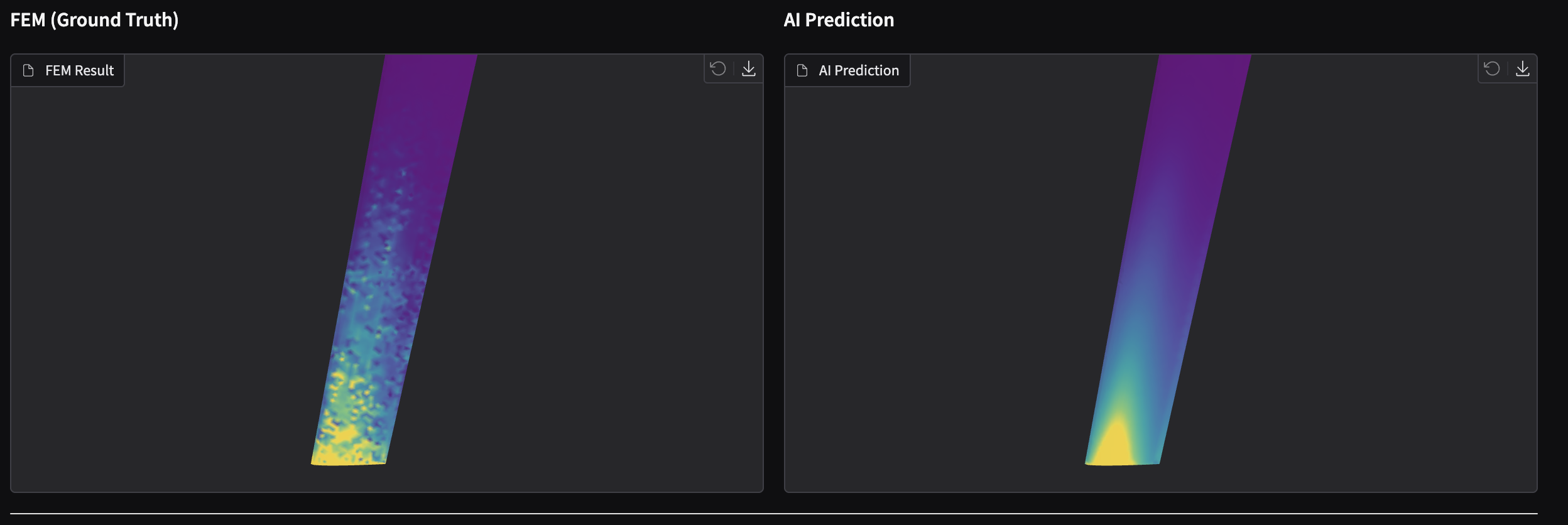
- FEM vs AI side-by-side comparison: Unified colormap (viridis, 98th percentile normalization)
Left: FEM simulation (Ground Truth) / Right: AI prediction (GraphSAGE)
1) Stage 4 — Dataset Validation
Before training, I validated all 200 FEM cases to ensure data quality.
1-1) Validation checks
# Key validation criteria
checks = {
    "nan_inf": "No NaN or Inf values in stress/displacement",
    "stress_range": "Max stress within reasonable bounds (< 1 GPa)",
    "node_count": "Sufficient surface nodes (> 100)",
    "displacement": "Displacement magnitude reasonable (< 1m)",
}
1-2) Results
| Metric | Value |
|---|---|
| Total cases | 200 |
| Passed | 200 (100%) |
| Failed | 0 |
| Avg surface nodes | ~4,200 |
| Avg max stress | ~50 MPa |
All 200 cases passed validation. The dataset is clean and ready for training.
2) Stage 5 — GNN Training (GraphSAGE)
2-1) Why GraphSAGE?
For mesh-based surrogate modeling, the key question is: how do we represent irregular mesh topology?
| Approach | Pros | Cons |
|---|---|---|
| MLP (node-wise) | Simple | Ignores connectivity |
| CNN (voxelize) | Standard | Resolution loss, memory |
| GNN (graph) | Native mesh topology | More complex |
GraphSAGE was chosen because:
- Handles variable-size meshes naturally
- Aggregates neighbor information (stress depends on surrounding structure)
- Inductive: generalizes to unseen geometries
2-2) Graph construction
Each surface mesh becomes a PyG Data object:
Data(
    x=[N, 6],           # Node features: [x, y, z, nx, ny, nz]
    edge_index=[2, E],  # Edge connectivity (from mesh faces)
    y=[N, 1],           # Target: von Mises stress (normalized)
    loss_mask=[N],      # True for nodes outside root singularity band
)
Loss mask rationale: FEM produces artificially high stress at fixed boundaries (root singularity). We exclude nodes with y < 5% span from the loss calculation.
2-3) Model architecture
GraphSAGE (3 layers)
├── SAGEConv(6 → 128) + ReLU + Dropout(0.1)
├── SAGEConv(128 → 128) + ReLU + Dropout(0.1)
├── SAGEConv(128 → 128) + ReLU + Dropout(0.1)
└── Linear(128 → 1)
Key hyperparameters:
- Hidden dim: 128
- Layers: 3
- Dropout: 0.1
- Aggregation: mean
- Optimizer: Adam (lr=1e-3)
- Scheduler: ReduceLROnPlateau (patience=10)
2-4) Training setup
# Requires CUDA for reasonable training time
python scripts/train_gnn.py- Train/Val/Test split: 160/20/20 cases
- Epochs: 200 (early stopping patience=30)
- Loss: MSE on normalized stress (masked)
- Hardware: RTX A4000 (trained on Windows, inference on Mac)
2-5) Training results
Best epoch: 142
Train Loss: 0.0053
Val Loss:   0.0010
Test MAE:   0.79 MPa (masked)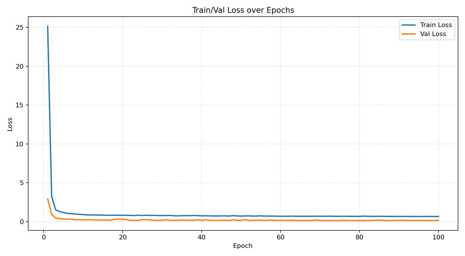
The model converged smoothly with no signs of overfitting (val loss < train loss).
3) Stage 6 — Inference + Visualization
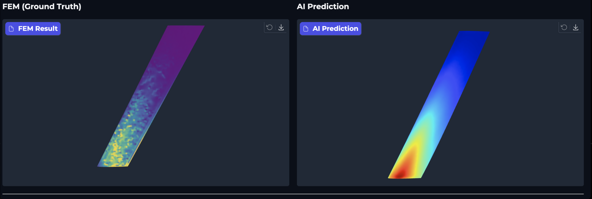
3-1) Unified colormap issue
Initial problem: FEM used viridis, AI used jet colormap. This made visual comparison misleading.
Before fix:
- FEM: viridis (purple → yellow)
- AI: jet (blue → red)
- Different color scales
After fix:
- Both use viridis
- Same normalization:
[min, 98th percentile]of FEM stress - Fair visual comparison
# Unified color scale: use GT (FEM) stress range
valid_gt = gt_stress[loss_mask]
vmin = float(np.min(valid_gt))
vmax = float(np.percentile(valid_gt, 98))  # 98th to avoid outlier domination

normalized = (pred_stress - vmin) / (vmax - vmin)
colors = viridis_colormap(normalized)
3-2) Deformation visualization issue
Another issue: AI wing appeared "bent" in the viewer.
Cause: I was applying displacement to AI visualization (deform_scale=10.0), but FEM visualization showed original geometry.
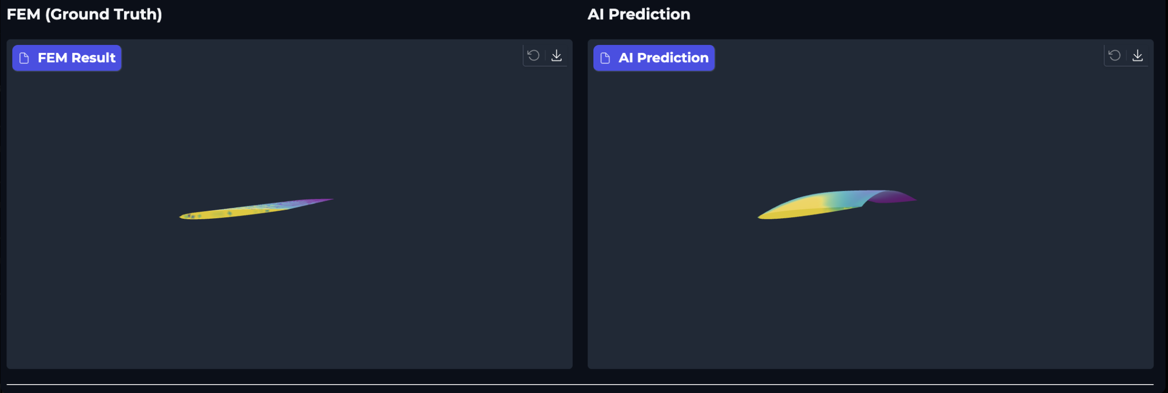
Fix: Use original pos for both FEM and AI GLBs. Deformation is only for engineering analysis, not comparison.
3-3) Gradio dashboard
The final dashboard provides:
- Side-by-side 3D viewer: FEM (left) vs AI (right)
- Engineering report: Geometry, material, stress metrics, safety factor
- AI accuracy metrics: MAE, RMSE, max error (all nodes / masked)
with gr.Blocks() as demo:
    gr.Markdown("# Deep-FEM-UAV-Wing")
    gr.Markdown("**FEM vs AI Comparison Dashboard**")

    with gr.Row():
        with gr.Column():
            gr.Markdown("### FEM (Ground Truth)")
            fem_viewer = gr.Model3D()
        with gr.Column():
            gr.Markdown("### AI Prediction")
            ai_viewer = gr.Model3D()

    report = gr.Markdown()  # Engineering report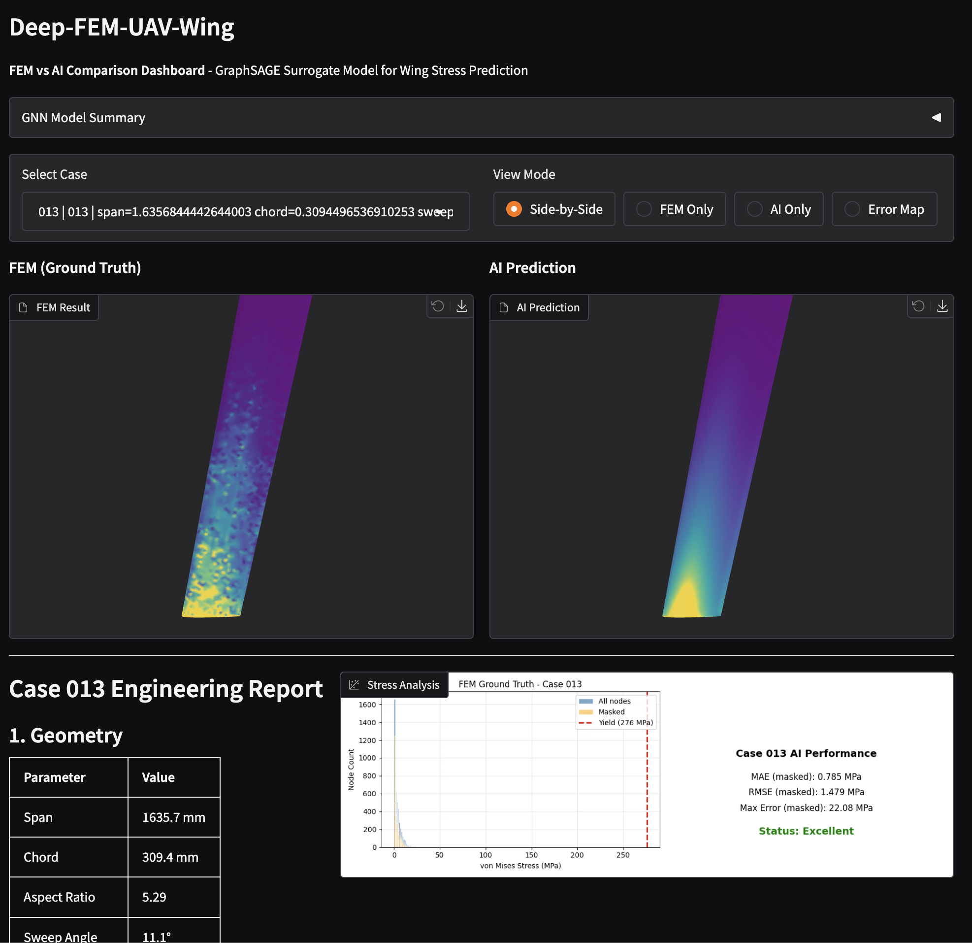
4) Performance Analysis
4-1) Overall metrics (200 cases)
| Metric | Value |
|---|---|
| MAE (masked) | 0.79 MPa |
| Relative error | ~3.3% of max stress |
| Val/Train loss ratio | 0.19 (no overfitting) |
| Inference time | ~0.1 sec/case (vs ~60 sec for FEM) |
4-2) Per-case analysis (Test set: Cases 001-005)
| Case | Masked MAE | FEM Max (MPa) | AI Max (MPa) | Note |
|---|---|---|---|---|
| 001 | 1.99 MPa | 134.2 | 37.0 | Peak underestimated |
| 002 | 1.02 MPa | 178.4 | 14.0 | Peak underestimated |
| 003 | 0.61 MPa | 49.4 | 17.7 | Good |
| 004 | 0.84 MPa | 26.8 | 13.2 | Good |
| 005 | 0.77 MPa | 118.2 | 10.9 | Peak underestimated |
4-3) Key finding: Peak stress underestimation
The most significant limitation is peak stress underestimation:
- Average stress: Well predicted (MAE ~0.79 MPa)
- Peak stress: Consistently underestimated (AI predicts ~30-50% of actual peak)
Why does this happen?
GraphSAGE aggregates neighbor information via mean pooling:
$$ h_v = W \cdot \text{MEAN}(\{h_u : u \in N(v)\}) $$
This averaging smooths out local extrema. Stress concentrations (high gradients) get diluted by surrounding lower-stress nodes.
4-4) Is this overfitting?
No. Evidence:
- Val loss (0.0010) < Train loss (0.0053)
- Test MAE consistent with validation MAE
- Model generalizes to unseen geometries
The peak underestimation is a structural limitation of mean-aggregation GNNs, not overfitting.
5) Limitations & Future Work
5-1) Current limitations
| Limitation | Impact | Mitigation |
|---|---|---|
| Peak underestimation | Safety factor overestimated | Use FEM for final verification |
| Training data bounds | Extrapolation unreliable | Restrict to trained geometry range |
| Single pressure value | Limited generalization | Train with variable pressure |
| Surface-only | No internal stress | Use volumetric GNN if needed |
5-2) Potential improvements
- Attention-based aggregation: Replace mean pooling with attention to preserve peaks
- GAT instead of GraphSAGE
- $h_v = \sum \alpha_{uv} \cdot W \cdot h_u$ (attention weights $\alpha$)
- Peak-weighted loss: Add penalty for peak stress error
- $\text{loss} = \text{MSE}(pred, gt) + \lambda \cdot |max(pred) - max(gt)|^2$
- Multi-scale architecture: Capture both local peaks and global distribution
``python # U-Net style encoder-decoder on graphs ``
- Physics-informed constraints: Add equilibrium/boundary condition losses
5-3) When to use this surrogate model
| Use case | Recommended? |
|---|---|
| Early design screening | ✅ Yes |
| Parameter sweep | ✅ Yes |
| Real-time optimization | ✅ Yes |
| Final safety verification | ❌ No (use FEM) |
| Regulatory certification | ❌ No (use FEM) |
6) Conclusion
What I built
An end-to-end pipeline for AI-based structural analysis prediction:
Blender → Gmsh → CalculiX → PyG → Gradio
(Geometry)  (Mesh)   (FEM)    (GNN)  (Dashboard)
Key achievements
- 200 cases generated, meshed, and solved automatically
- GraphSAGE surrogate trained with 0.79 MPa MAE
- 600x speedup (60s FEM → 0.1s AI)
- Side-by-side comparison dashboard for validation
Key lessons
- Data quality matters: Mesh consistency (winding, normals) caused many bugs
- Loss masking is essential: Root singularity would dominate training
- Visualization must match: Unified colormap/scale for fair comparison
- Know your limitations: GNN smoothing affects peak prediction
Final thoughts
Surrogate modeling is powerful for accelerating design iteration, but it's not a replacement for physics-based simulation. The key is knowing when each tool is appropriate.
For this project:
- AI: Fast screening, parameter exploration
- FEM: Final verification, safety-critical decisions
The code is available at: GitHub - Deep-FEM-UAV-Wing